This is Words and Buttons Online — a collection of interactive #tutorials, #demos, and #quizzes about #mathematics, #algorithms and #programming.
Mathematical analysis explained with Python , blood, and TNT
The key to understanding mathematical analysis is the word “analysis”. Nowadays it means “thinking really hard about something” but back in the XVII century, when mathematical analysis was invented, it was a lot closer to its original Greek meaning: “taking things apart”.
The most common type of analysis we all know is blood analysis. In the modern world, virtually everyone has to exchange a drop of blood for a sheet of numbers at least once in a while. What's interesting, the first step of the analysis is an actual separation. The blood gets taken apart into plasma, white blood cells, and red blood cells.
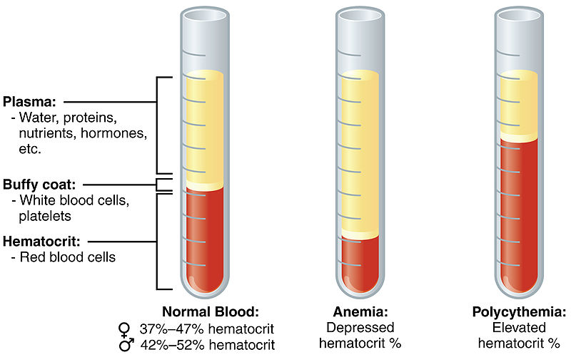
By OpenStax College [CC BY 3.0],
via Wikimedia Commons
There are different types of blood analyses. You can measure red cell count, cholesterol, hemoglobin, or even specific atomic substances such as sodium, potassium, or iron. Every measurement implies segregating the measurable substance from the rest of the input material. It doesn't necessarily mean physical separation. For instance, red blood cell count can be done by literally counting red blood cells under the microscope. But essentially analysis is still about taking things apart.
Mathematical analysis is also about taking things apart. Specifically, functions. But what are the functions' parts?
Derivative
For instance, you can separate a function into its derivatives. A derivative of a function f(x) in some x is a measure of how function changes in its neighborhood. It's like function's velocity, except you don't really have a speedometer for functions. So what do you do when you don't have a speedometer? You divide how far you go to the time it takes.
So in function's language, you do something like this:
| f(x + dx) - f(x) |
| dx |
It sure measures something. The problem is, if you take your dx big, the function may change its mind and go in another direction. It goes shorter “distance” during the same “time” and you wouldn't get the precise “velocity” measure. Here is the interactive plot that explains the problem.
Click anywhere to change dx.
The smaller dx is, the more accurate your measurements will be. With the magic of limits, you can get yourself a dx that is virtually smaller than any number. It is not a real number anymore, but a separate operable entity so usually derivatives are written slightly different from the usual division. Like this:
| d | f(x) |
| dx |
At any particular point, the derivative of a function is a number. If the function doesn't change its velocity, the number stays constant. But if it does, and of course all the most interesting functions do, it changes from point to point while forming some pattern. Here's the interactive plot that shows how it works with several popular functions.
Select a function and drag anywhere to leave marks.
You should have noticed that the patterns, the derivatives make, do look like functions on their own. That's because they are. The derivative of a function is a function. It is not always continuous, it is not even always defined, but in the general case it is true: the derivative of a function is a function.
And some of them are quite fascinating. The derivative of sine is cosine. The derivative of the logarithm is the inverse function. The derivative of the exponent is the exponent itself. And most importantly, the derivative of a polynomial is also a polynomial, only of decremented degree.
There are some quite elaborate rules to find the derivatives as functions. It usually takes about a semester to get moderately good in simple functional computations. It may be a fascinating experience on its own, but you don't really have to master calculus if you only want to calculate a few derivatives every now and then.
Getting derivatives as functions with SymPy
If you are not a practicing mathematician, you should be fine with automated tools for symbolic mathematics. Probably the most available of which is SymPy. It is available on-line, so you don't even have to install anything: SymPy Live.
SymPy is a Python library, but don't worry if you're not familiar with the language. We only need one word of it, so you don't really have to know Python to do some meaningful work with SymPy. Let's say we have a function:
y = x3 - 2x2 + 3x - 4
All we have to do to get its derivative with SymPy is to write it in a Python manner and run a diff. Like this:
>>> diff(x**3 - 2*x**2 + 3*x - 4, x)
3*x**2 - 4*x + 3
If you choose Str as the output format, the result is also calculable Python formula. You can put it back to diff to get the second, and then the third derivatives.
>>> diff(x**3 - 2*x**2 + 3*x - 4, x)
3*x**2 - 4*x + 3

>>> diff(3*x**2 - 4*x + 3, x)
6*x - 4

>>> diff(6*x - 4, x)
6
Of course, you don't have to manually copy the string just to get to the third derivative. You can just ask the SymPy to do it for you:
>>> diff(x*x*x - 2*x*x + 3*x - 4, x, 3)
6
It's as simple as that!
SymPy is in all ways amazing, it does all kind of symbolical computations for you. It does derivatives, integrals, equations, simplifications, and many more. And getting started with it is as easy as typing one function.
But back to the mathematics. What we just did here is we analyzed the polynomial into all its derivatives. It was the third-degree polynomial, so it had exactly 3 non-zero derivatives. But why did we do that? What is it good for? This can be answered in many ways, and one of them would be: to synthesize things alike.
Mathematical synthesis
The antonym for “analysis” is “synthesis” which means making things out of parts. Mathematical analysis as a domain of knowledge also covers the mathematical synthesis, which may seem confusing at first, but makes perfect sense when you see the duality of these things.
However, the most known field for synthesis is not mathematics but chemistry. We synthesize plastics, drugs, fertilizers, paint, and explosives. Chemical synthesis is a type of reaction when something complex appears out of simple compounds. Like TNT out of toluol, nitric acid, and oleum.

On the low level, TNT consists of only 4 primitive substances: carbon, hydrogen, oxygen, and nitrogen.
Now the blood, we mentioned before as an analysis subject, is much more complex than TNT. It's not a mono-molecular substance, it has a very complex biological structure. Every blood cell is as complex as any mono-cellular life form. It also carries your full DNA so technically it's at least as complex as you are.
We can't synthesize blood chemically. We can do substitutes that work reasonably well as oxygen transport, but we can't synthesize blood. It's just too complex.
However, what we can do is we can extract some minuscule quantity of nitrogen from the blood. Also carbon and hydrogen. And oxygen obviously. So, while we can't just take a drop of blood, analyze it into chemical compounds, and then put it back together, we technically (and I mean technically, not ethically or even technologically) can make TNT out of it.
The same principle works in mathematics too. We can't always synthesize the exact function we want, but we can provide a substitute for it. Or something that will blow up in our faces.
Polynomial series
Let's start with something familiar. Like the polynomial from before.
f(x) = x3 - 2x2 + 3x - 4
The easiest point to calculate f(x) in is x = 0. If x is 0 then x3 is 0, and 2x2 is 0, and 3x is 0. f(0) = -4.
The first derivative of f(x), as we established with SymPy, is:
f'(x) = 3x2 - 4x + 3
By the same logic f'(0) = 3. Then the second derivative:
f"(x) = 6x - 4
And f"(0) = -4. The last third derivative is just a number 6, so f'''(0) = 6.
So, we analyzed the polynomial to the set of its derivatives in 0. Including the original value they are: [-4, 3, -4, 6]. Now let's synthesize it back.
You might have noticed that when you get a derivative of a single term you decrement its x's power but multiply its coefficient to the power decremented.
| d | axn | = | naxn-1 |
| dx |
That also means that:
- the n'th derivative of that very term is a number, since x0 = 1;
- this number is an! since it's the product of all decrements of n.
And, more importantly, this means that we can reconstruct our polynomial term by term out of its derivatives in 0:
- the last coefficient will remain -4;
- the one before last will be 3/1! which is, of course, 3;
- the one before that will be -4/2! that is -2;
- and the first one: 6/3! that is 1.
Not really impressive, is it? We took a polynomial apart and glued it back. There is not much point in this exercise. But we can do more than the polynomials in this very way.
Polynomials are especially interesting in this regard because functions don't usually run out of derivatives just like that. Functions like sine or exponent have an infinite number of derivatives, so we can't just disassemble them completely. But we can try to analyze (almost) any function into a finite series of numbers and then take it back as a polynomial. Usually, the more derivatives we count, the more precise our polynomial will mimic the original function.
Why is this important? One reason would be, computers don't know trigonometry. They don't know logarithms or exponents either, they are basically summators on steroids. They can do multiplication reasonably fast, but that's it. Fortunately, with polynomial series that's all we need! We only need summation and multiplication to calculate a polynomial.
Of course, this is not the ultimate solution. For instance, polynomials are quite good substitutes for trigonometric functions, but they are only substitutes. There is always a question of precision. Luckily, all of our computations in floating-point numbers are imprecise, so usually, we can get away by making our series just marginally more precise than the carrier type.
And there is always the more serious problem of representability. Remember “almost” from before? We can't actually represent every function we want, for the very least the logarithm is not determined in 0 at all. There is no log(0) and that upsets our scheme. We can cheat it out by synthesizing log(1-x). But even though, the model we'll get will only be plausible on a certain interval.
Here is a plot with some most known serializable functions. Feel free to explore.
Conclusion
Of course, the mathematical analysis doesn't end here. In college it takes a couple of semesters to master the basics of it, so even considering the shortcuts, it simply can't be comprehensibly exposed in one small piece of words and buttons. However, I hope this piece shows you the reason people are willing to spend years studying it. It's not only about polynomial series. Splines, approximations, extrapolations, differential equations, the largest part of mathematical modeling is based on the analysis. It's very a pragmatic thing to learn, although it is incredibly dull when you only do exercises and don't even see how it pays off in the end.
But it does. If anything, the analysis is the most stable educational investment. You can do more money with the <insert any currently over-hyped technology here> in the short run, but the expertise in it will expire in some 10 or 20 years, while the expertise in analysis is still valuable four centuries after its invention.
| Index #mathematics #tutorials | ← there's more. |
+ Github & RSS |